Using row reduction to solve a system of equations is a fundamental topic in linear algebra, used in everything from physics and engineering to economics and computer science.
While there are multiple methods for solving these systems—such as substitution, elimination, and matrix inversion—row reduction (also known as Gaussian elimination) is one of the most efficient and systematic approaches.
Row reduction transforms a system of equations into a simpler form, making it easier to identify solutions.
By converting a system’s augmented matrix into Row Echelon Form (REF) or Reduced Row Echelon Form (RREF), we can quickly determine whether the system has a unique solution, infinitely many solutions, or no solution at all.
If you’re looking for a step-by-step way to solve matrices using row reduction, an interactive calculator like matrixrowreductioncalculator.com can speed up the process and help you verify your work.
If you’re new to the concepts of Row Echelon Form vs. Reduced Row Echelon Form, check out our previous post, Row Echelon Form vs Reduced Row Echelon Form, for a detailed breakdown of their differences.
In this guide, we’ll go through how to use row reduction to solve the system of equations, with step-by-step examples to illustrate the process. Let’s get started!
Representing a System of Equations as a Matrix
Before we begin row reduction, we first need to represent our system of equations in matrix form.
This is done using an augmented matrix, which allows us to apply row operations systematically.
What is an Augmented Matrix?
An augmented matrix is a compact way of writing a system of linear equations. It consists of:
- The coefficient matrix (which contains the coefficients of the variables).
- A column of constants (which represents the right-hand side of the equations).
This format allows us to apply row operations directly to the entire system without rewriting the equations repeatedly.
Example: Converting a System of Equations into an Augmented Matrix
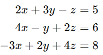
Consider the following system of equations:
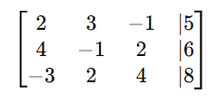
We extract the coefficients and constants to form the augmented matrix:
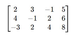
The vertical bar separates the coefficients from the constants, but in actual calculations, it’s often omitted:
By writing our system in this format, we can now apply row reduction techniques to simplify the matrix and solve for x, y, and z.
If you want to skip manual calculations, you can enter your system into an online tool like MatrixRowReductionCalculator.com to instantly convert it into row echelon or reduced row echelon form.
Next, we’ll dive into the step-by-step process of using row operations to solve the system! 🚀
Row Reduction Process (Gaussian and Gauss-Jordan Elimination)
Now that we have our system represented as an augmented matrix, we can begin the row reduction process. There are two common methods for solving a system using row operations:
- Gaussian Elimination: This method reduces the matrix to Row Echelon Form (REF). From there, we use back-substitution to solve for the variables.
- Gauss-Jordan Elimination: This method goes a step further by reducing the matrix to Reduced Row Echelon Form (RREF), where the solution can be read directly without back-substitution.
If you’re not familiar with the differences between REF and RREF, check out our previous blog post, Row Echelon Form vs Reduced Row Echelon Form for a detailed comparison.
Let’s go step by step through the row reduction process.
Step 1: Convert to Row Echelon Form (REF)
To achieve REF, we apply the following row operations:
- Make the first pivot (leading coefficient) a 1 by scaling the row if necessary.
- Use row operations to make all values below the pivot equal to 0.
- Move to the next pivot position and repeat the process.
For example, transforming this matrix:
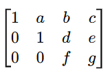
into row echelon form might look like this:
where a, b, c, d, e, f, g are the transformed values.
At this stage, we could use back-substitution to solve for the variables.
If you need a refresher on how to reach Row Echelon Form, check out our blog post, Row Echelon Form Examples 3×3 – Step by Step Solutions for more examples.
Step 2: Convert to Reduced Row Echelon Form (RREF)
To reach RREF, we continue with additional row operations:
- Make all values above each leading 1 equal to 0.
- Ensure each leading 1 is the only nonzero value in its column.
Applying these steps transforms the REF matrix into:
Now, the values x, y , x, and z are the solutions to the system.
If you’re looking for a quick way to reach RREF without manual calculations, use MatrixRowReductionCalculator.com to enter your augmented matrix and get instant results.
Step 3: Interpret the Solution from the Final Matrix
Once the matrix is in REF or RREF, we can determine the type of solution:
- Unique Solution: If each variable has a leading 1 and there are no contradictory rows, the system has a single solution (x, y, z).
- Infinitely Many Solutions: If there is at least one free variable (a column without a leading 1), the system has infinitely many solutions, often expressed in parametric form.
- No Solution: If a row reduces to an inconsistency (e.g., [0 0 0 1]), the system is inconsistent and has no solution.
To get more hands-on practice, try solving different systems using our step-by-step matrix row reduction guide.
Now that we’ve covered the row reduction process, let’s see how this method applies in real-world problem solving! 🚀
Use Row Reduction to Solve the System of Equations For Different Types of Systems
When solving a system of equations using row reduction, we can encounter three possible outcomes:
- A Unique Solution (Full Rank)
- Infinitely Many Solutions (Dependent Equations)
- No Solution (Inconsistent System)
Let’s go through each case with examples to understand how to interpret the results.
1. Unique Solution Case (Full Rank)
A system has a unique solution when the number of independent equations matches the number of variables.
This means that, after row reduction, the matrix reaches Reduced Row Echelon Form (RREF) with each variable having a leading 1 in a distinct row.
Example:
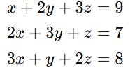
Consider this system:
Its augmented matrix is:
After row reduction, we get:
Since every variable has a leading 1 in a separate row, we can directly read the unique solution (x, y, z).
This is called a full-rank system, meaning the number of independent equations equals the number of variables.
2. Infinite Solutions Case (Dependent Equations)
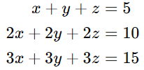
A system has infinitely many solutions when one or more rows become dependent (i.e., they do not contribute new information). This happens when there are fewer independent equations than variables.
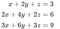
Example:
Consider this system:
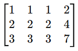
Its augmented matrix is:
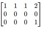
After row reduction, we get:
Since the bottom two rows are all zeros, the system has one free variable, leading to infinitely many solutions. We express the solution in parametric form using the free variable.
This occurs because the second and third equations are multiples of the first, making them redundant.
3. No Solution Case (Inconsistent System)
A system has no solution when row reduction results in an inconsistency, such as a row that translates to an equation like 0 = 1.
This means the system is contradictory and does not have any values for x, y, x, and z that satisfy all equations.
Example:
Consider this system:
Its augmented matrix is:
After row reduction, we get:
Since the last row translates to 0 = 1, which is a contradiction, the system is inconsistent, meaning there is no solution.
Using a Calculator to Identify Solution Types
If you want to quickly determine whether a system has a unique solution, infinitely many solutions, or no solution, you can use matrixrowreductioncalculator.com.
Simply enter your augmented matrix, and the tool will reduce it to REF or RREF, allowing you to interpret the result instantly.
For more examples and detailed step-by-step guides, check out:
Example Problems with Step-by-Step Solutions
To solidify your understanding of solving systems of equations using row reduction, let’s go through three examples:
- A simple 2×2 system with a unique solution.
- A 3×3 system with a unique solution.
- A 3×3 system with infinite solutions.
For each example, we will convert the system into an augmented matrix and perform row reduction step by step.
Example 1: Simple 2×2 System (Unique Solution)
Solve the system using row reduction:
Step 1: Convert to an Augmented Matrix

Step 2: Perform Row Reduction
- Multiply row 1 by -2 and add it to row 2:

- Divide row 2 by -3 to make the pivot 1:

- Subtract row 2 from row 1:

Solution:
![]()
Example 2: 3×3 System (Unique Solution)
Solve the system:
Step 1: Convert to an Augmented Matrix
Step 2: Row Reduce to REF
- Subtract 2 × row 1 from row 2.
- Subtract 3 × row 1 from row 3.
- Multiply row 2 by -1 to make the pivot positive:
- Add 5 × row 2 to row 3:
- Divide row 3 by 18 to get a leading 1:
- Subtract 5 × row 3 from row 2.
- Subtract 3 × row 3 from row 1.
- Subtract 2 × row 2 from row 1:

Example 3: 3×3 System (Infinite Solutions)
Solve the system:
Step 1: Convert to an Augmented Matrix
Step 2: Perform Row Reduction
- Subtract 2 × row 1 from row 2.
- Subtract 3 × row 1 from row 3.
Step 3: Interpret the Result
The second and third rows are all zeros, meaning we have one equation with two free variables:
![]()
Let y = t and z = s where t and s can be any real numbers. Then, solving for xx:
![]()
Solution:
![]()
This means there are infinitely many solutions. ✅
Try Solving Your Own Systems!
Want to practice more? Use the Matrix Row Reduction Calculator to input any system and get step-by-step solutions.
Now that you’ve seen these examples, let’s look at row reduction is applied in real life. 🚀
Applications of Row Reduction in Real Life
Row reduction is more than just a mathematical exercise—it plays a crucial role in solving real-world problems across various fields.
Here are some key areas where row reduction is widely used:
1. Engineering ⚙️
Engineers use systems of equations to analyze electrical circuits, structural forces, and control systems. Row reduction helps:
- Solve Kirchhoff’s circuit equations to determine current and voltage.
- Analyze mechanical stress in bridges and buildings.
- Optimize control systems for robotics and automation.
2. Physics 🔬
Linear algebra is essential in physics, where row reduction is used to:
- Solve motion equations in classical mechanics.
- Analyze quantum states in quantum mechanics.
- Model electromagnetic field equations in Maxwell’s laws.
3. Data Science and Machine Learning 📊
In modern computing, row reduction is a fundamental tool for:
- Solving linear regression problems in predictive modeling.
- Reducing data dimensions using principal component analysis (PCA).
- Optimizing algorithms in artificial intelligence and deep learning.
4. Economics and Finance 💰
Economists and financial analysts use row reduction to:
- Solve supply and demand models for market equilibrium.
- Optimize investment portfolios using linear programming.
- Analyze economic forecasts based on multiple variables.
Try It Yourself!
Want to see how row reduction works in action? Use the Matrix Row Reduction Calculator to test different matrices and solve real-world problems!
Now, let’s wrap up with some key takeaways! 🚀
Conclusion
In this post we learned how to use row reduction to solve the system of equations.
Row reduction is a powerful and efficient method.
Generally, by converting a system into an augmented matrix and applying Gaussian or Gauss-Jordan elimination, we can determine whether a system has a unique solution, infinitely many solutions, or no solution at all.
Furthermore, understanding row reduction not only helps in solving mathematical problems, but also has real-world applications in engineering, physics, data science, and economics.
Finally, whether you’re working on a school assignment or tackling complex computational problems, mastering this technique is a valuable skill.
To practice and explore different matrices, try using the Matrix Row Reduction Calculator for step-by-step solutions.
For more detailed guides, check out:
With a solid grasp of row reduction, you can confidently solve linear systems and apply these concepts to more advanced topics in mathematics and beyond!











Be First to Comment